
These studies appear in Workbench → Models → Structural models and in the exercise collection. Each runs separately from coupled process or progressive analyses. Reference-state results are exploratory; analytical software checks do not establish experimentally validated design allowables.
01 · Open-hole strength
Infinite-width, specially orthotropic tension screening. Point and average stress distances must be calibrated independently for this laminate. Not compression, bearing or a joint allowable.
Model tree location, inputs and result handoff ↗
Equations, calibration and limits
σ(r)/σ∞ = 1 + ½q² + 3/2 q⁴ − ½(Kt − 3)(5q⁶ − 7q⁸), q = a/r.
For loading along x, Kt = 1 + √[2(√(Ex/Ey) − νxy) + Ex/Gxy]. The point criterion evaluates stress at a + d₀; the average criterion integrates it from a to a + a₀. Both compare with measured unnotched laminate strength. Their two characteristic lengths need independent calibration. The isotropic limit is Kt = 3.
NASA: notch-strength modelling and characteristic-distance assumptions ↗
Exercise workflow and model layers
Linked-input preview, not solved results. Gray blocks are not configured.
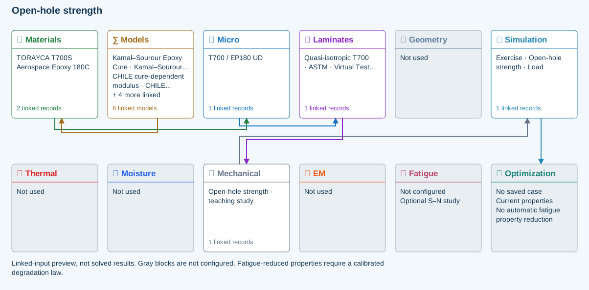
∑ Selected models & submodels
These are the exercise’s linked choices, not solved results. Open a first-layer model to see its submodels and scope.
Kamal–Sourour autocatalytic · Kamal–Sourour Epoxy Cure
Reusable material model. It contributes only when assigned to a material used by this simulation; separate model records can supply independent properties.
Calibration & applicability
Illustrative model defaults — replace with characterized resin kinetics
CHILE (degree of cure) · CHILE cure-dependent modulus
Reusable material model. It contributes only when assigned to a material used by this simulation; separate model records can supply independent properties. Cure-dependent modulus does not automatically scale strength allowables.
Calibration & applicability
CHILE(α), section 2.4 of Materials 2019, 12, 259. Example parameters, not measured EP180 data. Fixed Poisson ratio; no viscoelastic relaxation or Tg softening. Incremental elastic stress integration at saved process intervals: check time-step convergence. Strength allowables are independent measured inputs, not scaled with modulus.
Temperature-dependent tabular · Temperature-dependent Thermal
Reusable material model. It contributes only when assigned to a material used by this simulation; separate model records can supply independent properties. Micro uses the 23 °C reference; Process evaluates the same table at local temperature, without extrapolation.
Calibration & applicability
Check source data, applicable environment and validity limits in the model record; saved defaults are not experimental validation.
1D Fickian diffusion · Layered Fickian Diffusion
Reusable material model. It contributes only when assigned to a material used by this simulation; separate model records can supply independent properties.
Calibration & applicability
Check source data, applicable environment and validity limits in the model record; saved defaults are not experimental validation.
Halpin–Tsai · T700 / EP180 UD
One compatible homogenization model per Micro recipe. Separate recipes compare models; their predictions are not blended.
∑ Theory & assumptionsWhitney–Nuismer open-hole tension · Open-hole strength · teaching study
Infinite-width, specially orthotropic tension screening. Point and average stress distances must be calibrated independently for this laminate. Not compression, bearing or a joint allowable.
Linked laminate reference state
Ply stiffness, thickness and orientation come from the linked laminate. Other thermal or structural analyses must be run separately.
Calibration & study controls
Teaching example
Hole radius: 3 mm
Unnotched tensile strength: 500 MPa
Measured laminate strength, not fiber strength.
Point stress distance: 1 mm
Average stress distance: 2 mm
Remote tensile stress: 100 MPa
Data travelling between blocks
Micro → Laminates
Predicted ply stiffness, strength, density and expansion properties.
Materials → Micro
Constituent stiffness, strength, density and thermal / moisture properties.
Models → Materials
Model choices and calibrated parameters.
Mechanical → Simulation
SIMULATION selects this case and its analysis model; the case owns its applicable cycle and input references.
Laminates → Mechanical
Ply angles and thicknesses, stiffness, mass and ply properties.
Simulation → Optimization
Linked inputs and current-property response for candidate evaluation.
02 · Creep & stress relaxation
Linear uniaxial response at the calibration temperature. Reference Ex is the instantaneous modulus. Three Maxwell branches; creep is solved from stress equilibrium, not the reciprocal relaxation modulus. No thermal shifting or nonlinear creep.
Model tree location, inputs and result handoff ↗
Equations, calibration and limits
E(t) = E∞ + Σ Eᵢ exp(−t/τᵢ), E∞ = E₀(1 − Σgᵢ).
The laminate reference Ex is E₀. A held-strain experiment gives stress relaxation. For held stress, the solver evolves Maxwell branch stresses and solves equilibrium for strain; creep compliance is not 1/E(t). The calculation compares two time refinements and rejects excessive differences. Three editable branches, one calibration temperature, small uniaxial strain.
Exercise workflow and model layers
Linked-input preview, not solved results. Gray blocks are not configured.
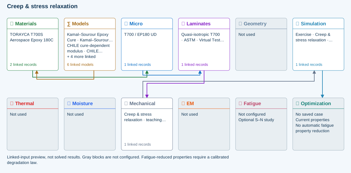
∑ Selected models & submodels
These are the exercise’s linked choices, not solved results. Open a first-layer model to see its submodels and scope.
Kamal–Sourour autocatalytic · Kamal–Sourour Epoxy Cure
Reusable material model. It contributes only when assigned to a material used by this simulation; separate model records can supply independent properties.
Calibration & applicability
Illustrative model defaults — replace with characterized resin kinetics
CHILE (degree of cure) · CHILE cure-dependent modulus
Reusable material model. It contributes only when assigned to a material used by this simulation; separate model records can supply independent properties. Cure-dependent modulus does not automatically scale strength allowables.
Calibration & applicability
CHILE(α), section 2.4 of Materials 2019, 12, 259. Example parameters, not measured EP180 data. Fixed Poisson ratio; no viscoelastic relaxation or Tg softening. Incremental elastic stress integration at saved process intervals: check time-step convergence. Strength allowables are independent measured inputs, not scaled with modulus.
Temperature-dependent tabular · Temperature-dependent Thermal
Reusable material model. It contributes only when assigned to a material used by this simulation; separate model records can supply independent properties. Micro uses the 23 °C reference; Process evaluates the same table at local temperature, without extrapolation.
Calibration & applicability
Check source data, applicable environment and validity limits in the model record; saved defaults are not experimental validation.
1D Fickian diffusion · Layered Fickian Diffusion
Reusable material model. It contributes only when assigned to a material used by this simulation; separate model records can supply independent properties.
Calibration & applicability
Check source data, applicable environment and validity limits in the model record; saved defaults are not experimental validation.
Halpin–Tsai · T700 / EP180 UD
One compatible homogenization model per Micro recipe. Separate recipes compare models; their predictions are not blended.
∑ Theory & assumptionsGeneralized Maxwell · axial Prony · Creep & stress relaxation · teaching study
Linear uniaxial response at the calibration temperature. Reference Ex is the instantaneous modulus. Three Maxwell branches; creep is solved from stress equilibrium, not the reciprocal relaxation modulus. No thermal shifting or nonlinear creep.
Linked laminate reference state
Ply stiffness, thickness and orientation come from the linked laminate. Other thermal or structural analyses must be run separately.
Calibration & study controls
Teaching example
Relaxation fraction 1: 0.15 —
Relaxation time 1: 10 s
Relaxation fraction 2: 0.2 —
Relaxation time 2: 100 s
Relaxation fraction 3: 0.1 —
Relaxation time 3: 1000 s
Study duration: 1000 s
Held axial stress: 10 MPa
Held axial strain: 0.001 —
Calibration temperature: 23 °C
Data travelling between blocks
Micro → Laminates
Predicted ply stiffness, strength, density and expansion properties.
Materials → Micro
Constituent stiffness, strength, density and thermal / moisture properties.
Models → Materials
Model choices and calibrated parameters.
Mechanical → Simulation
SIMULATION selects this case and its analysis model; the case owns its applicable cycle and input references.
Laminates → Mechanical
Ply angles and thicknesses, stiffness, mass and ply properties.
Simulation → Optimization
Linked inputs and current-property response for candidate evaluation.
03 · Analytical bonded joint
Identical equivalent-elastic adherends, long free arms and a thin elastic adhesive. Compare shear-only Volkersen with eccentric single-lap shear and peel. Not a debonding, plasticity or strength calculation.
Model tree location, inputs and result handoff ↗
Equations, calibration and limits
Volkersen: τ(x) = (F/b) β cosh(βx) / [2 sinh(βL/2)].
β² = 2Ga/(ta Et) for identical adherends. The companion Goland–Reissner solution adds the eccentric-load moment factor and elastic peel distribution. The shared laminate supplies thickness and Ex, with an equivalent-isotropic beam approximation. Adhesive modulus, Poisson ratio, thickness, width and overlap remain explicit study inputs. Peak elastic stress is not a joint-strength prediction.
University of Washington: Goland–Reissner calculation equations ↗
Exercise workflow and model layers
Linked-input preview, not solved results. Gray blocks are not configured.
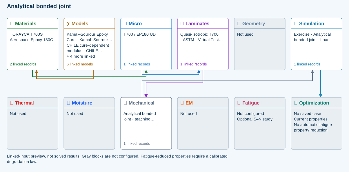
∑ Selected models & submodels
These are the exercise’s linked choices, not solved results. Open a first-layer model to see its submodels and scope.
Kamal–Sourour autocatalytic · Kamal–Sourour Epoxy Cure
Reusable material model. It contributes only when assigned to a material used by this simulation; separate model records can supply independent properties.
Calibration & applicability
Illustrative model defaults — replace with characterized resin kinetics
CHILE (degree of cure) · CHILE cure-dependent modulus
Reusable material model. It contributes only when assigned to a material used by this simulation; separate model records can supply independent properties. Cure-dependent modulus does not automatically scale strength allowables.
Calibration & applicability
CHILE(α), section 2.4 of Materials 2019, 12, 259. Example parameters, not measured EP180 data. Fixed Poisson ratio; no viscoelastic relaxation or Tg softening. Incremental elastic stress integration at saved process intervals: check time-step convergence. Strength allowables are independent measured inputs, not scaled with modulus.
Temperature-dependent tabular · Temperature-dependent Thermal
Reusable material model. It contributes only when assigned to a material used by this simulation; separate model records can supply independent properties. Micro uses the 23 °C reference; Process evaluates the same table at local temperature, without extrapolation.
Calibration & applicability
Check source data, applicable environment and validity limits in the model record; saved defaults are not experimental validation.
1D Fickian diffusion · Layered Fickian Diffusion
Reusable material model. It contributes only when assigned to a material used by this simulation; separate model records can supply independent properties.
Calibration & applicability
Check source data, applicable environment and validity limits in the model record; saved defaults are not experimental validation.
Halpin–Tsai · T700 / EP180 UD
One compatible homogenization model per Micro recipe. Separate recipes compare models; their predictions are not blended.
∑ Theory & assumptionsVolkersen & Goland–Reissner joint · Analytical bonded joint · teaching study
Identical equivalent-elastic adherends, long free arms and a thin elastic adhesive. Compare shear-only Volkersen with eccentric single-lap shear and peel. Not a debonding, plasticity or strength calculation.
Linked laminate reference state
Ply stiffness, thickness and orientation come from the linked laminate. Other thermal or structural analyses must be run separately.
Calibration & study controls
Teaching example
Overlap length: 25 mm
Joint width: 25 mm
Adhesive thickness: 0.2 mm
Adhesive modulus: 2000 MPa
Adhesive Poisson ratio: 0.35 —
Joint tensile force: 1000 N
Data travelling between blocks
Micro → Laminates
Predicted ply stiffness, strength, density and expansion properties.
Materials → Micro
Constituent stiffness, strength, density and thermal / moisture properties.
Models → Materials
Model choices and calibrated parameters.
Mechanical → Simulation
SIMULATION selects this case and its analysis model; the case owns its applicable cycle and input references.
Laminates → Mechanical
Ply angles and thicknesses, stiffness, mass and ply properties.
Simulation → Optimization
Linked inputs and current-property response for candidate evaluation.
04 · LaRC04 failure initiation
NASA LaRC04 linear-shear specialization, evaluated at both faces of every ply under membrane and bending loads. Supplied ply strengths are effective/in-situ values; no automatic thin-ply enhancement. Initiation only, not degradation or nonlinear-shear instability.
Model tree location, inputs and result handoff ↗
Equations, calibration and limits
LaRC04 evaluates matrix tension/compression and fiber tension/kinking in their appropriate fracture and misalignment frames.
This release implements the linear-shear specialization of NASA Table 6. CLT recovers stress at both faces of each ply; the kink-frame rotation solves the linear shear equilibrium equation and the fracture-plane search is refined. Supply effective/in-situ strengths explicitly. Identical ply materials share one calibration; mixed-material calibration is rejected. This separate initiation study does not replace or silently extend the progressive-failure solver. Nonlinear-shear instability and delamination are excluded.
Pinho et al., NASA/TM-2005-213530: original LaRC04 equations ↗
Exercise workflow and model layers
Linked-input preview, not solved results. Gray blocks are not configured.
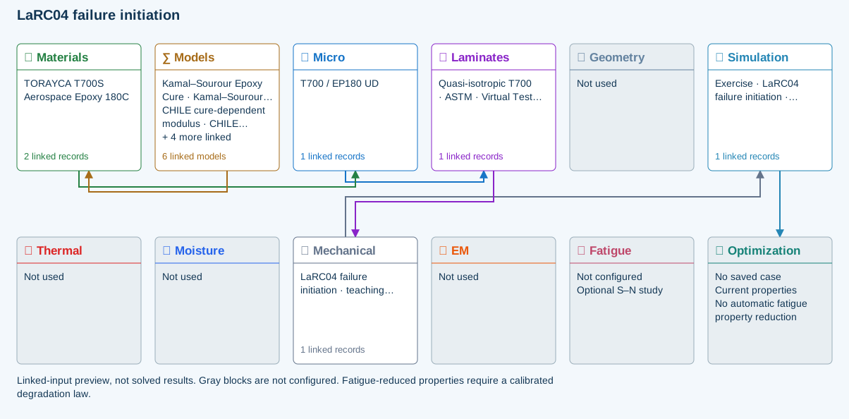
∑ Selected models & submodels
These are the exercise’s linked choices, not solved results. Open a first-layer model to see its submodels and scope.
Kamal–Sourour autocatalytic · Kamal–Sourour Epoxy Cure
Reusable material model. It contributes only when assigned to a material used by this simulation; separate model records can supply independent properties.
Calibration & applicability
Illustrative model defaults — replace with characterized resin kinetics
CHILE (degree of cure) · CHILE cure-dependent modulus
Reusable material model. It contributes only when assigned to a material used by this simulation; separate model records can supply independent properties. Cure-dependent modulus does not automatically scale strength allowables.
Calibration & applicability
CHILE(α), section 2.4 of Materials 2019, 12, 259. Example parameters, not measured EP180 data. Fixed Poisson ratio; no viscoelastic relaxation or Tg softening. Incremental elastic stress integration at saved process intervals: check time-step convergence. Strength allowables are independent measured inputs, not scaled with modulus.
Temperature-dependent tabular · Temperature-dependent Thermal
Reusable material model. It contributes only when assigned to a material used by this simulation; separate model records can supply independent properties. Micro uses the 23 °C reference; Process evaluates the same table at local temperature, without extrapolation.
Calibration & applicability
Check source data, applicable environment and validity limits in the model record; saved defaults are not experimental validation.
1D Fickian diffusion · Layered Fickian Diffusion
Reusable material model. It contributes only when assigned to a material used by this simulation; separate model records can supply independent properties.
Calibration & applicability
Check source data, applicable environment and validity limits in the model record; saved defaults are not experimental validation.
Halpin–Tsai · T700 / EP180 UD
One compatible homogenization model per Micro recipe. Separate recipes compare models; their predictions are not blended.
∑ Theory & assumptionsLaRC04 · linear shear · LaRC04 failure initiation · teaching study
NASA LaRC04 linear-shear specialization, evaluated at both faces of every ply under membrane and bending loads. Supplied ply strengths are effective/in-situ values; no automatic thin-ply enhancement. Initiation only, not degradation or nonlinear-shear instability.
Linked laminate reference state
Ply stiffness, thickness and orientation come from the linked laminate. Other thermal or structural analyses must be run separately.
Calibration & study controls
Teaching example
Fiber tensile strength: 1500 MPa
Fiber compressive strength: 900 MPa
Matrix tensile strength: 50 MPa
Matrix compressive strength: 200 MPa
Longitudinal shear strength: 75 MPa
Fracture angle: 53 deg
Fracture toughness ratio: 0.35 —
Data travelling between blocks
Micro → Laminates
Predicted ply stiffness, strength, density and expansion properties.
Materials → Micro
Constituent stiffness, strength, density and thermal / moisture properties.
Models → Materials
Model choices and calibrated parameters.
Mechanical → Simulation
SIMULATION selects this case and its analysis model; the case owns its applicable cycle and input references.
Laminates → Mechanical
Ply angles and thicknesses, stiffness, mass and ply properties.
Simulation → Optimization
Linked inputs and current-property response for candidate evaluation.
05 · Tool-release shape
Free CLT release from prescribed ply-local shrinkage/thermal eigenstrains. Corner spring-in is a separate uniform-strain estimate. Stress-free temperature and effective post-gel shrinkage need calibration. No tool friction, cure kinetics or viscoelastic restraint history.
Model tree location, inputs and result handoff ↗
Equations, calibration and limits
[ε₀, κ]ᵀ = ABD⁻¹[N*, M*]ᵀ; Δθ = θ(εparallel − εthrough)/(1 + εthrough).
The first expression computes free flat-laminate response to prescribed ply-local thermal and post-gel shrinkage strains. The second is a separate uniform-strain corner estimate; positive Δθ means spring-in. The plotted free sections use their center tangent as reference, not a clamp. Enter effective post-gel strains, not total resin volumetric shrinkage. Tool friction, contact and viscoelastic cure history are not resolved.
Exercise workflow and model layers
Linked-input preview, not solved results. Gray blocks are not configured.
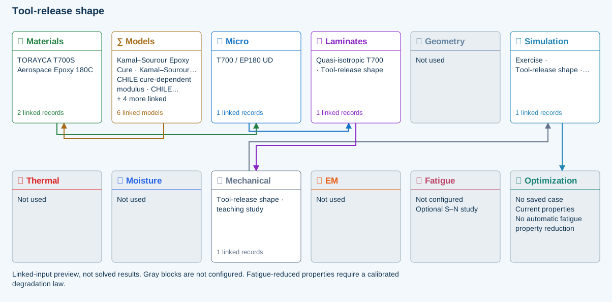
∑ Selected models & submodels
These are the exercise’s linked choices, not solved results. Open a first-layer model to see its submodels and scope.
Kamal–Sourour autocatalytic · Kamal–Sourour Epoxy Cure
Reusable material model. It contributes only when assigned to a material used by this simulation; separate model records can supply independent properties.
Calibration & applicability
Illustrative model defaults — replace with characterized resin kinetics
CHILE (degree of cure) · CHILE cure-dependent modulus
Reusable material model. It contributes only when assigned to a material used by this simulation; separate model records can supply independent properties. Cure-dependent modulus does not automatically scale strength allowables.
Calibration & applicability
CHILE(α), section 2.4 of Materials 2019, 12, 259. Example parameters, not measured EP180 data. Fixed Poisson ratio; no viscoelastic relaxation or Tg softening. Incremental elastic stress integration at saved process intervals: check time-step convergence. Strength allowables are independent measured inputs, not scaled with modulus.
Temperature-dependent tabular · Temperature-dependent Thermal
Reusable material model. It contributes only when assigned to a material used by this simulation; separate model records can supply independent properties. Micro uses the 23 °C reference; Process evaluates the same table at local temperature, without extrapolation.
Calibration & applicability
Check source data, applicable environment and validity limits in the model record; saved defaults are not experimental validation.
1D Fickian diffusion · Layered Fickian Diffusion
Reusable material model. It contributes only when assigned to a material used by this simulation; separate model records can supply independent properties.
Calibration & applicability
Check source data, applicable environment and validity limits in the model record; saved defaults are not experimental validation.
Halpin–Tsai · T700 / EP180 UD
One compatible homogenization model per Micro recipe. Separate recipes compare models; their predictions are not blended.
∑ Theory & assumptionsFree-release eigenstrain & spring-in · Tool-release shape · teaching study
Free CLT release from prescribed ply-local shrinkage/thermal eigenstrains. Corner spring-in is a separate uniform-strain estimate. Stress-free temperature and effective post-gel shrinkage need calibration. No tool friction, cure kinetics or viscoelastic restraint history.
Linked laminate reference state
Ply stiffness, thickness and orientation come from the linked laminate. Other thermal or structural analyses must be run separately.
Calibration & study controls
Teaching example
Stress-free temperature: 180 °C
Release temperature: 23 °C
Axial CTE: 0 1/K
Transverse CTE: 0.00003 1/K
Through-thickness CTE: 0.00005 1/K
Axial cure shrinkage: 0 —
Signed strain: negative means contraction.
Transverse cure shrinkage: -0.002 —
Through-thickness cure shrinkage: -0.005 —
Corner angle: 90 deg
Shape length: 25 mm
Data travelling between blocks
Micro → Laminates
Predicted ply stiffness, strength, density and expansion properties.
Materials → Micro
Constituent stiffness, strength, density and thermal / moisture properties.
Models → Materials
Model choices and calibrated parameters.
Mechanical → Simulation
SIMULATION selects this case and its analysis model; the case owns its applicable cycle and input references.
Laminates → Mechanical
Ply angles and thicknesses, stiffness, mass and ply properties.
Simulation → Optimization
Linked inputs and current-property response for candidate evaluation.
06 · Fatigue residual properties
Prescribed power-law retention fitted to constant-amplitude tests at a fixed stress ratio, amplitude and temperature. Stiffness and strength have independent coefficients. S–N life alone cannot calibrate either. Does not modify the saved laminate.
Model tree location, inputs and result handoff ↗
Equations, calibration and limits
E(N)/E₀ = 1 − aE(N/Nf)^bE; X(N)/X₀ = 1 − aX(N/Nf)^bX.
This is a prescribed, user-fitted phenomenological retention law. Stiffness and strength use independent loss fractions and exponents. Nf, stress ratio, peak stress and temperature must describe the same constant-amplitude calibration. No extrapolation beyond Nf is allowed. Curves do not automatically modify the saved laminate, and S–N life alone cannot determine degradation coefficients. The reference illustrates why stiffness-degradation data are needed; CDS does not claim to reproduce that NASA fitted model.
NASA: measured stiffness degradation for fatigue prognosis ↗
Exercise workflow and model layers
Linked-input preview, not solved results. Gray blocks are not configured.
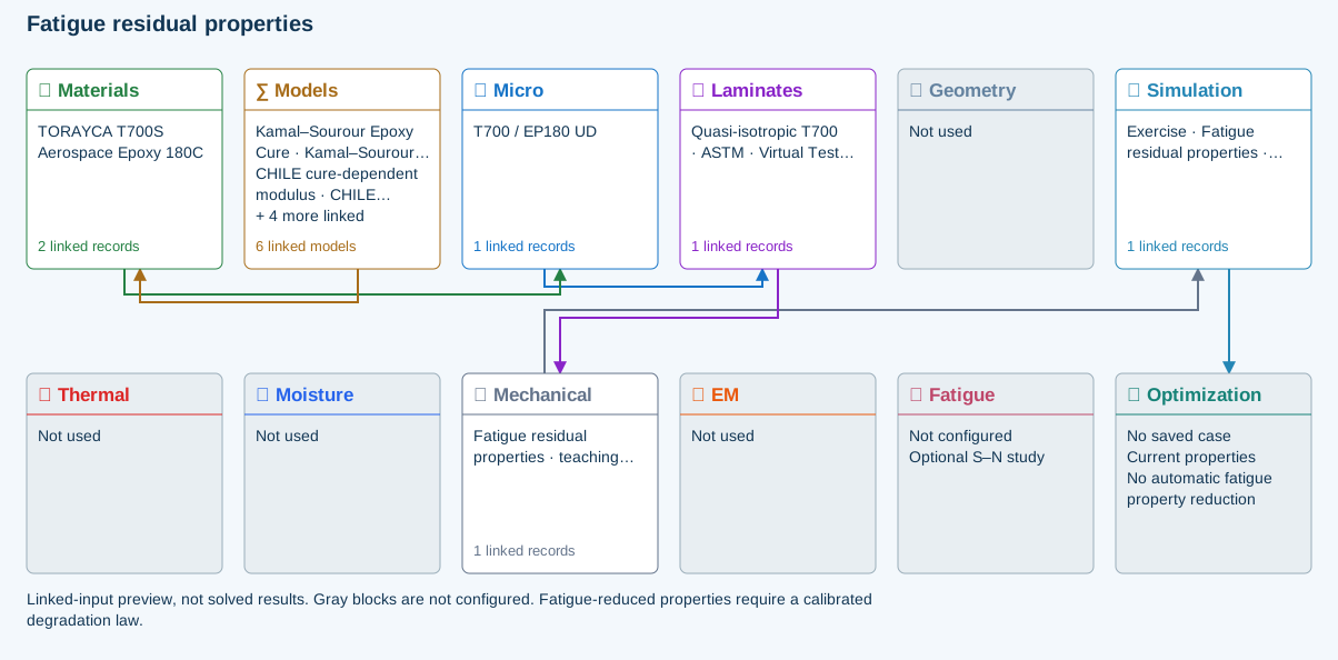
∑ Selected models & submodels
These are the exercise’s linked choices, not solved results. Open a first-layer model to see its submodels and scope.
Kamal–Sourour autocatalytic · Kamal–Sourour Epoxy Cure
Reusable material model. It contributes only when assigned to a material used by this simulation; separate model records can supply independent properties.
Calibration & applicability
Illustrative model defaults — replace with characterized resin kinetics
CHILE (degree of cure) · CHILE cure-dependent modulus
Reusable material model. It contributes only when assigned to a material used by this simulation; separate model records can supply independent properties. Cure-dependent modulus does not automatically scale strength allowables.
Calibration & applicability
CHILE(α), section 2.4 of Materials 2019, 12, 259. Example parameters, not measured EP180 data. Fixed Poisson ratio; no viscoelastic relaxation or Tg softening. Incremental elastic stress integration at saved process intervals: check time-step convergence. Strength allowables are independent measured inputs, not scaled with modulus.
Temperature-dependent tabular · Temperature-dependent Thermal
Reusable material model. It contributes only when assigned to a material used by this simulation; separate model records can supply independent properties. Micro uses the 23 °C reference; Process evaluates the same table at local temperature, without extrapolation.
Calibration & applicability
Check source data, applicable environment and validity limits in the model record; saved defaults are not experimental validation.
1D Fickian diffusion · Layered Fickian Diffusion
Reusable material model. It contributes only when assigned to a material used by this simulation; separate model records can supply independent properties.
Calibration & applicability
Check source data, applicable environment and validity limits in the model record; saved defaults are not experimental validation.
Halpin–Tsai · T700 / EP180 UD
One compatible homogenization model per Micro recipe. Separate recipes compare models; their predictions are not blended.
∑ Theory & assumptionsCalibrated residual-property fatigue · Fatigue residual properties · teaching study
Prescribed power-law retention fitted to constant-amplitude tests at a fixed stress ratio, amplitude and temperature. Stiffness and strength have independent coefficients. S–N life alone cannot calibrate either. Does not modify the saved laminate.
Linked laminate reference state
Ply stiffness, thickness and orientation come from the linked laminate. Other thermal or structural analyses must be run separately.
Calibration & study controls
Teaching example
Calibrated fatigue life: 1000000 cycles
Elapsed cycles: 500000 cycles
Stiffness loss at life: 0.3 —
Stiffness exponent: 1.5 —
Strength loss at life: 0.5 —
Strength exponent: 1 —
Initial residual strength: 500 MPa
Calibration stress ratio: 0.1 —
Calibration peak stress: 200 MPa
Calibration temperature: 23 °C
Data travelling between blocks
Micro → Laminates
Predicted ply stiffness, strength, density and expansion properties.
Materials → Micro
Constituent stiffness, strength, density and thermal / moisture properties.
Models → Materials
Model choices and calibrated parameters.
Mechanical → Simulation
SIMULATION selects this case and its analysis model; the case owns its applicable cycle and input references.
Laminates → Mechanical
Ply angles and thicknesses, stiffness, mass and ply properties.
Simulation → Optimization
Linked inputs and current-property response for candidate evaluation.
07 · Cylinder buckling
Simply supported, thin, specially orthotropic cylinder under uniform axial compression. Discrete Donnell modes; prescribed knockdown factor explores imperfection sensitivity, not a prediction from measured imperfection amplitude. No pressure, torsion, postbuckling or strength pass.
Model tree location, inputs and result handoff ↗
Equations, calibration and limits
Nx,cr = [D11 k⁴ + 2(D12 + 2D66)k²l² + D22 l⁴ + k⁴/(R²C)] / k².
Here k = mπ/L, l = n/R and C = a22k⁴ + (2a12 + a66)k²l² + a11l⁴, with a = A⁻¹. The solver searches discrete axial and circumferential modes for a thin, specially orthotropic simply supported cylinder. A governing mode at the search boundary requires refinement. An explicit knockdown factor scales the ideal result; it is not an automatic prediction from measured imperfections. Pressure, torsion, postbuckling and failure interaction are excluded.
Exercise workflow and model layers
Linked-input preview, not solved results. Gray blocks are not configured.
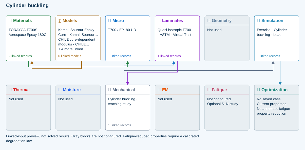
∑ Selected models & submodels
These are the exercise’s linked choices, not solved results. Open a first-layer model to see its submodels and scope.
Kamal–Sourour autocatalytic · Kamal–Sourour Epoxy Cure
Reusable material model. It contributes only when assigned to a material used by this simulation; separate model records can supply independent properties.
Calibration & applicability
Illustrative model defaults — replace with characterized resin kinetics
CHILE (degree of cure) · CHILE cure-dependent modulus
Reusable material model. It contributes only when assigned to a material used by this simulation; separate model records can supply independent properties. Cure-dependent modulus does not automatically scale strength allowables.
Calibration & applicability
CHILE(α), section 2.4 of Materials 2019, 12, 259. Example parameters, not measured EP180 data. Fixed Poisson ratio; no viscoelastic relaxation or Tg softening. Incremental elastic stress integration at saved process intervals: check time-step convergence. Strength allowables are independent measured inputs, not scaled with modulus.
Temperature-dependent tabular · Temperature-dependent Thermal
Reusable material model. It contributes only when assigned to a material used by this simulation; separate model records can supply independent properties. Micro uses the 23 °C reference; Process evaluates the same table at local temperature, without extrapolation.
Calibration & applicability
Check source data, applicable environment and validity limits in the model record; saved defaults are not experimental validation.
1D Fickian diffusion · Layered Fickian Diffusion
Reusable material model. It contributes only when assigned to a material used by this simulation; separate model records can supply independent properties.
Calibration & applicability
Check source data, applicable environment and validity limits in the model record; saved defaults are not experimental validation.
Halpin–Tsai · T700 / EP180 UD
One compatible homogenization model per Micro recipe. Separate recipes compare models; their predictions are not blended.
∑ Theory & assumptionsDonnell cylinder · axial buckling · Cylinder buckling · teaching study
Simply supported, thin, specially orthotropic cylinder under uniform axial compression. Discrete Donnell modes; prescribed knockdown factor explores imperfection sensitivity, not a prediction from measured imperfection amplitude. No pressure, torsion, postbuckling or strength pass.
Linked laminate reference state
Ply stiffness, thickness and orientation come from the linked laminate. Other thermal or structural analyses must be run separately.
Calibration & study controls
Teaching example
Shell mean radius: 100 mm
Shell length: 500 mm
Axial compression resultant: 100 N/mm
Imperfection knockdown factor: 0.65 —
Mode search limit: 40 —
Data travelling between blocks
Micro → Laminates
Predicted ply stiffness, strength, density and expansion properties.
Materials → Micro
Constituent stiffness, strength, density and thermal / moisture properties.
Models → Materials
Model choices and calibrated parameters.
Mechanical → Simulation
SIMULATION selects this case and its analysis model; the case owns its applicable cycle and input references.
Laminates → Mechanical
Ply angles and thicknesses, stiffness, mass and ply properties.
Simulation → Optimization
Linked inputs and current-property response for candidate evaluation.
08 · Uncertainty & sensitivity
Seeded independent uniform sampling of shared modulus, ply-thickness and angle offsets. Recomputes laminate ABD for each sample. Bounds are assumptions, not measured distributions. Percentiles and sensitivity are exploratory, not reliability certification.
Model tree location, inputs and result handoff ↗
Equations, calibration and limits
For each seeded sample: vary bounded inputs → rebuild ABD → solve the axial response.
Sampled independent uniform inputs are a common modulus scale, a common thickness scale and a shared ply-angle offset. The output includes strain percentiles and signed Pearson correlations. Repeating the same seed and inputs reproduces the sample set. Zero input ranges recover the deterministic result. Distributions must be justified before drawing reliability conclusions; a small correlation does not rule out nonlinear influence.
Exercise workflow and model layers
Linked-input preview, not solved results. Gray blocks are not configured.
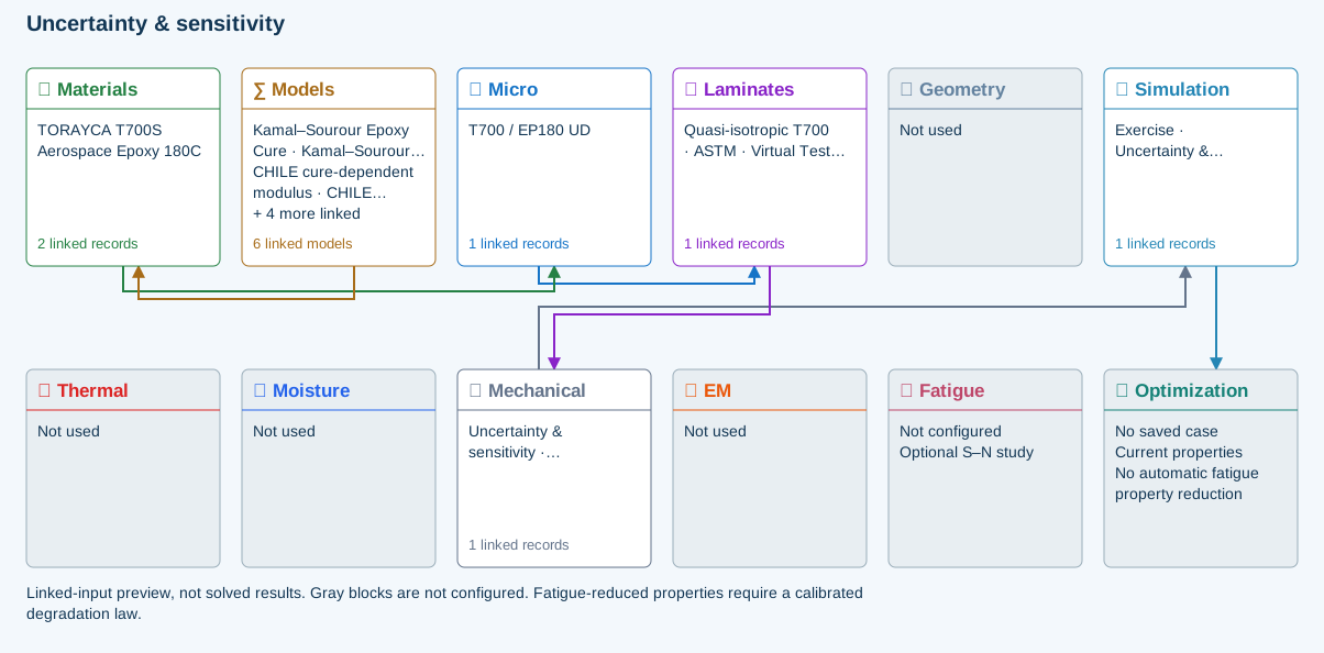
∑ Selected models & submodels
These are the exercise’s linked choices, not solved results. Open a first-layer model to see its submodels and scope.
Kamal–Sourour autocatalytic · Kamal–Sourour Epoxy Cure
Reusable material model. It contributes only when assigned to a material used by this simulation; separate model records can supply independent properties.
Calibration & applicability
Illustrative model defaults — replace with characterized resin kinetics
CHILE (degree of cure) · CHILE cure-dependent modulus
Reusable material model. It contributes only when assigned to a material used by this simulation; separate model records can supply independent properties. Cure-dependent modulus does not automatically scale strength allowables.
Calibration & applicability
CHILE(α), section 2.4 of Materials 2019, 12, 259. Example parameters, not measured EP180 data. Fixed Poisson ratio; no viscoelastic relaxation or Tg softening. Incremental elastic stress integration at saved process intervals: check time-step convergence. Strength allowables are independent measured inputs, not scaled with modulus.
Temperature-dependent tabular · Temperature-dependent Thermal
Reusable material model. It contributes only when assigned to a material used by this simulation; separate model records can supply independent properties. Micro uses the 23 °C reference; Process evaluates the same table at local temperature, without extrapolation.
Calibration & applicability
Check source data, applicable environment and validity limits in the model record; saved defaults are not experimental validation.
1D Fickian diffusion · Layered Fickian Diffusion
Reusable material model. It contributes only when assigned to a material used by this simulation; separate model records can supply independent properties.
Calibration & applicability
Check source data, applicable environment and validity limits in the model record; saved defaults are not experimental validation.
Halpin–Tsai · T700 / EP180 UD
One compatible homogenization model per Micro recipe. Separate recipes compare models; their predictions are not blended.
∑ Theory & assumptionsSeeded laminate uncertainty · Uncertainty & sensitivity · teaching study
Seeded independent uniform sampling of shared modulus, ply-thickness and angle offsets. Recomputes laminate ABD for each sample. Bounds are assumptions, not measured distributions. Percentiles and sensitivity are exploratory, not reliability certification.
Linked laminate reference state
Ply stiffness, thickness and orientation come from the linked laminate. Other thermal or structural analyses must be run separately.
Calibration & study controls
Teaching example
Sample count: 200 —
Random seed: 2026 —
Modulus half-range: 0.1 —
Thickness half-range: 0.05 —
Angle half-range: 3 deg
Axial resultant: 100 N/mm
Data travelling between blocks
Micro → Laminates
Predicted ply stiffness, strength, density and expansion properties.
Materials → Micro
Constituent stiffness, strength, density and thermal / moisture properties.
Models → Materials
Model choices and calibrated parameters.
Mechanical → Simulation
SIMULATION selects this case and its analysis model; the case owns its applicable cycle and input references.
Laminates → Mechanical
Ply angles and thicknesses, stiffness, mass and ply properties.
Simulation → Optimization
Linked inputs and current-property response for candidate evaluation.
Verification before interpretation
Reference checks cover isotropic notch concentration, exact one-branch creep, joint load transfer, pure-load LaRC04 initiation, zero-curvature free expansion, fatigue-retention endpoints, classical isotropic shell buckling and seeded deterministic sampling. Check the scope of each model and repeat sensitivity/convergence studies for your actual inputs. A completed calculation is not an overall design pass.
Workbench availability: released models, inputs and compatible study paths. The wider theory library includes reference formulations not available in every Workbench solve.