Prepare, visualize, optimize, and run
analysis cases.

Choose the run in the SIMULATION block

SIMULATION is the control point for the run. Select a Thermal case, Moisture case, Mechanical case and EM case, or None in any slot. Each selected case shows its analysis model, laminate and applicable geometry.

1. Keep candidate records in the surrounding blocks. Adding a candidate does not select it for execution.
2. Select the required cases in SIMULATION and review their inputs before Run. At least one case is required.
3. Use the same laminate for a supported combined run. Run standalone studies separately with the other selectors set to None.
4. Run executes the selected combination. A connection or Used marker is not evidence of a successful solve.

Review every downstream geometry dependency

A geometry record can be shared by several cases and simulations. Editing its dimensions or type affects all linked consumers, including studies that are not currently open. Unrelated records are unchanged.

1. After editing geometry, open Solver messages and expand Review affected cases and simulations. Select a linked name to inspect that record.
2. Check the selected model, load basis, dimensions and boundary conditions. Loads are not automatically replaced when the geometry changes.
3. Resolve incompatible geometry and model combinations before running. An I-section does not turn a plate theory into a beam theory.
4. Rerun affected simulations before relying on previous results. Inputs changed warnings indicate that stored results no longer match their connected inputs.

Read the blue Used marker

Connected, available record selections have a soft blue glow and a Used marker in the corner. Hover or focus the marker to see which downstream record and field uses that input.

1. Check the marker before editing a shared input: more than one case can consume it.
2. A Used marker means connected, not solved or validated. Review solver status and outdated-result warnings separately.
3. Missing or incompatible selections need repair; do not interpret an empty result as zero response.

Add, replace or disconnect a block input

The + control adds another available record to a block, excluding records already present. Use that record row dropdown to change the candidate, its link to open it, and − to remove it from the block. Library records are not deleted.

1. Choose + and search for a compatible candidate not already in the block. Decide what actually runs with the four selectors in SIMULATION.
2. If no compatible record exists, create one in Inputs. Each case owns its analysis model and applicable cycle. There is no separate Process block to connect.
3. A used input must first be disconnected or changed at its consuming field. Review downstream warnings before confirming a removal; cancel to keep it.
4. After removal, required missing inputs remain flagged and their selectors allow reconnection. Optional cases may stay disconnected. Rerun affected analyses before relying on their results.

Create a case with its own cycle

Choose a Thermal, Moisture, Mechanical or EM case. Each case selects one analysis model and owns its applicable conditions and cycle. There is no separate Process block.

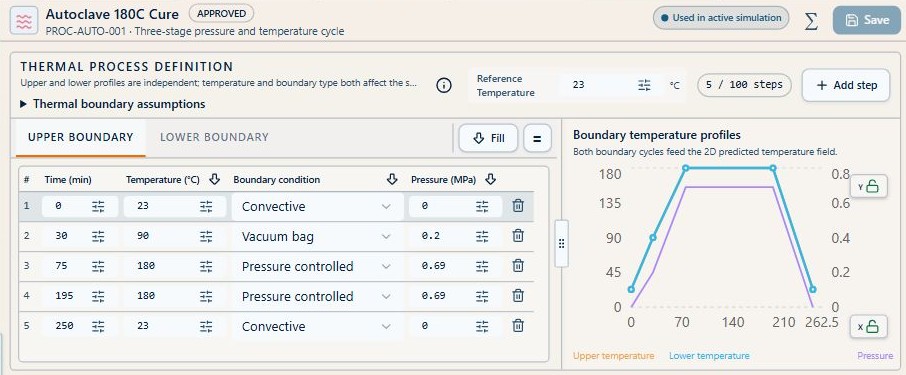
Edit the cycle inside the case

In a thermal case, use Initial conditions for analysis setup and the Upper and Lower tabs for independent surface schedules. Set each surface condition and film coefficient in this case. Moisture and mechanical schedules belong to their own cases and do not share the thermal cycle.

1. Enter monotonically increasing time values. See screenshot
2. Enter temperature and pressure for each step. See screenshot
3. Set upper and lower boundary types and values. See screenshot
4. Inspect the plot beside the table for discontinuities or unit errors. See screenshot

Assemble a simulation input record

In SIMULATION select Thermal, Moisture, Mechanical and EM cases, each with None available. The other blocks hold used and available records. Check the model, laminate and applicable geometry beneath each selected case.

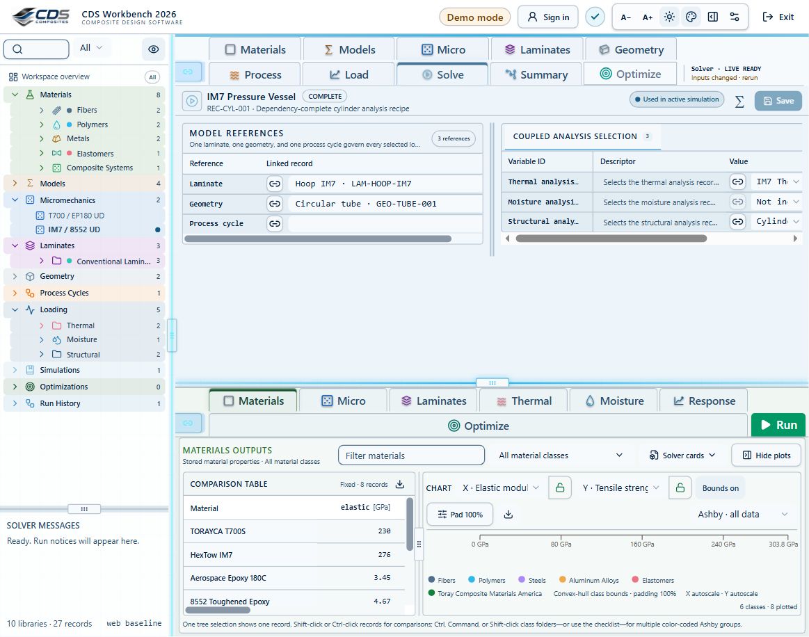
Review the LiveLoad schematic

The LiveLoad block appears beside Loads and Thermal inputs for analysis cases. Its plate, cylinder, or thermal schematic updates with the selected geometry, boundary conditions, loads, and directions. A zero-valued load vector is greyed so active loading is immediately recognizable.

Run the model

Resolve missing selections, invalid numbers, broken references, invalid ply angles, and zero laminate thickness before choosing Run. Use the Simulation workflow for a final dependency and model check.

1. Confirm the LiveLoad schematic matches the intended model.
2. Keep the desired Results tab selected. See screenshot
3. Choose Run when required; the interface preserves that tab while the model executes. See screenshot
4. Review result values, freshness and solver messages.

Understand solver provenance

Workbench uses its embedded production solver when no external solver endpoint is configured. When an external endpoint is configured, a timeout, rejected request or incompatible response is reported as an error; it is not silently replaced by a successful fallback result.

Check thermal setup and accuracy

A thermal result needs a compatible thermal case model, linked laminate, transport properties, initial conditions and its embedded cycle where required by that model. Missing setup is not a zero-temperature result.

1. Follow the missing-setup message to the linked source record rather than interpreting an empty plot.
2. After upstream edits, rerun before using a saved temperature, cure or moisture history.
3. Refine through-thickness resolution and review temperature gradients and numerical diagnostics.
4. Output spacing controls saved samples; it is not the integration accuracy target. The transient solver checks full-step/two-half-step agreement.

Include cure exotherm and evolving modulus

Transient thermal analysis can include the heat released by cure. The selected cure-dependent modulus model then changes the stiffness used to develop process stress as degree of cure evolves.

1. Assign a cure-kinetics model, total heat of reaction, density and heat capacity to the material or ply.
2. Enable cure exotherm when the thermal solution should include reaction heat; leave it off for externally imposed thermal histories that intentionally exclude self-heating. See screenshot
3. Assign the cure-dependent modulus model and review its editable transition, rubbery/glassy modulus and shape parameters.
4. Rerun after changing kinetics, transport, cure heat, modulus evolution or shrinkage. These inputs affect later residual-stress and failure results.

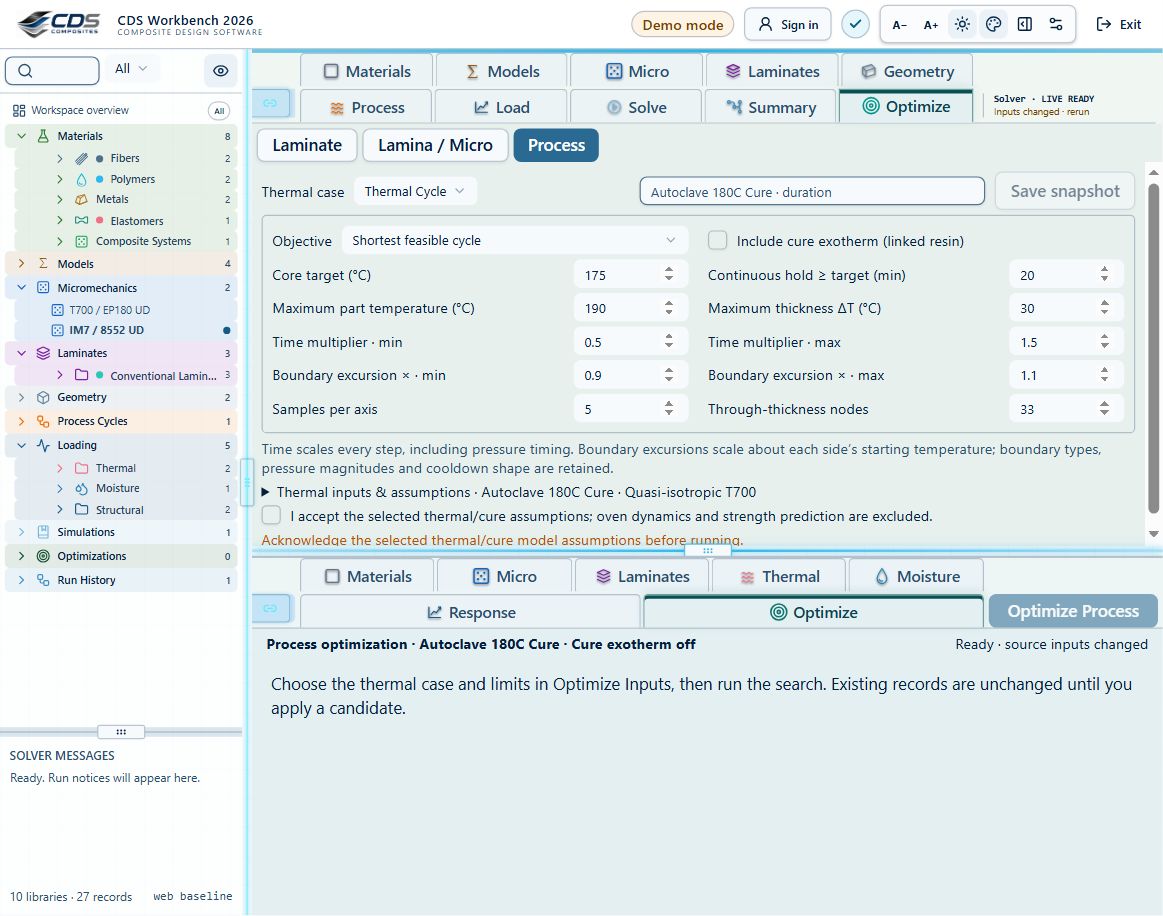
Optimize an oven or process cycle

Process optimization varies selected surface-cycle controls to meet a target core temperature or cure state while reducing time, overshoot or other configured penalties.

1. Choose Process in Optimize Inputs and select the thermal case and its laminate. Review the cycle owned by that case. See screenshot
2. Choose a target such as core temperature, degree of cure, maximum temperature difference, overshoot or total cycle time. See screenshot
3. Select the editable boundary variables—surface temperatures, ramp rates, dwell temperatures or dwell durations—and define bounds and constraints. See screenshot
4. Choose steady-state only for equilibrium targets. Use transient mode for ramps, dwells, core lag, cure exotherm, evolving modulus and stress development.
5. Run the bounded search, inspect feasibility and convergence, save a snapshot, then apply the candidate to the case-owned cycle and review the resulting case.
6. Rerun the full coupled simulation before accepting residual stress, distortion or failure results from the optimized cycle.