Keep the model connected
and the result traceable.

Inspect the selected model in Live Sim

SIMULATE opens with Live Sim, an input-driven view of the selected cases. The four selectors remain available above the scene. Switch to Blocks to manage candidate records and trace their connections.

1. Select Geometry, Laminate, a constituent or a case to inspect the inputs that are actually used. Clicking a used block heading also opens its Live Sim inspection.
2. Select a ply in the stack or geometry view to inspect its source. Micro-derived and stored-property plies are identified separately. Woven sources show the fabric unit-cell preview when applicable.
3. Select the Thermal or Moisture case to inspect its surface boundary schedule. Move the step slider to compare prescribed conditions. This is not a solved internal temperature or moisture field.
4. Use Edit input to open the source record. The scene follows the changed inputs; rerun the simulation before trusting previous results.

Use the current CASES database format

This release reads and saves the current CASES database format only. Thermal and Moisture schedules are stored directly with their cases. There is no separate Process record or old-format migration on opening a file.

1. Download a current starter or exercise database from the library. Older-format files are rejected with a clear message rather than converted silently.
2. Save and reopen the current database to retain case selections, schedules, candidate records and editable names.
3. Missing folders, duplicate identifiers and cycles attached to absent cases prevent saving or opening. Blank physical inputs remain editable and must be completed before Run.

Choose the run in the SIMULATION block

SIMULATION is the control point for the run. Select a Thermal case, Moisture case, Mechanical case and EM case, or None in any slot. Each selected case shows its analysis model, laminate and applicable geometry.

1. Keep candidate records in the surrounding blocks. Adding a candidate does not select it for execution.
2. Select the required cases in SIMULATION and review their inputs before Run. At least one case is required.
3. Use the same laminate for a supported combined run. Run standalone studies separately with the other selectors set to None.
4. Run executes the selected combination. A connection or Used marker is not evidence of a successful solve.

Review every downstream geometry dependency

A geometry record can be shared by several cases and simulations. Editing its dimensions or type affects all linked consumers, including studies that are not currently open. Unrelated records are unchanged.

1. After editing geometry, open Solver messages and expand Review affected cases and simulations. Select a linked name to inspect that record.
2. Check the selected model, load basis, dimensions and boundary conditions. Loads are not automatically replaced when the geometry changes.
3. Resolve incompatible geometry and model combinations before running. An I-section does not turn a plate theory into a beam theory.
4. Rerun affected simulations before relying on previous results. Inputs changed warnings indicate that stored results no longer match their connected inputs.

Build the simulation from interactive blocks

Choose Block view above the left navigator for a vertical, editable workflow, or Blocks inside SIMULATE for the larger connection view. Live Sim inspects the selected model. Record dropdowns remain visible in Lite view.

1. Choose the active simulation, then select compatible materials, Micro recipes, laminates, geometry and cases inside its blocks. Hybrid laminates can retain both stored-material and solved-Micro ply sources.
2. Use the local Blocks Lite–Advanced switch for extra details without changing the rest of the workspace. Existing search and current-simulation filters still apply.
3. Use the side connections to trace the input path. Hide connections or pause their animation locally; reduced-motion preferences are respected. Animation indicates connection direction, not solver progress.

Read the blue Used marker

Connected, available record selections have a soft blue glow and a Used marker in the corner. Hover or focus the marker to see which downstream record and field uses that input.

1. Check the marker before editing a shared input: more than one case can consume it.
2. A Used marker means connected, not solved or validated. Review solver status and outdated-result warnings separately.
3. Missing or incompatible selections need repair; do not interpret an empty result as zero response.

Add, replace or disconnect a block input

The + control adds another available record to a block, excluding records already present. Use that record row dropdown to change the candidate, its link to open it, and − to remove it from the block. Library records are not deleted.

1. Choose + and search for a compatible candidate not already in the block. Decide what actually runs with the four selectors in SIMULATION.
2. If no compatible record exists, create one in Inputs. Each case owns its analysis model and applicable cycle. There is no separate Process block to connect.
3. A used input must first be disconnected or changed at its consuming field. Review downstream warnings before confirming a removal; cancel to keep it.
4. After removal, required missing inputs remain flagged and their selectors allow reconnection. Optional cases may stay disconnected. Rerun affected analyses before relying on their results.

Keep starter laminates in one classification

Generated Standard starter Conventional Laminates folders are consolidated into the main Conventional Laminates folder. Distinct laminate record IDs and their simulation links are preserved; identical titles alone are not a reason to delete a record.

CASES organizes the conditions you apply

CASES is the Workbench section formerly called LOAD or Loading. Its four types are Thermal, Moisture, Mechanical and Electromagnetic. A case defines the model, conditions and linked inputs for one study; SIMULATE connects the cases into the supported workflow.

1. Choose the appropriate case type. Thermal and moisture cases use their compatible transport properties and boundary schedules; structural cases define forces, pressure, restraints or prescribed motion; EM cases define field, frequency and supported wave-study inputs.
2. Each case selects one analysis model and owns its applicable cycle. Configure thermal initial conditions and upper/lower surface schedules in that case; moisture and mechanical schedules remain separate. Select cases in SIMULATION, not a separate Process block.
3. Use an existing case or create one, check its laminate, geometry and model, then apply it to the current simulation. Review missing-input messages before running.

Test section stiffness during cure

The x–z section can use the linked matrix’s CHILE cure-dependent modulus, with the Micro recipe recomputing longitudinal, transverse and shear stiffnesses through the thickness.

1. Link cure kinetics and a cure-modulus model to the matrix used by the Micro recipe. All section plies must use that same recipe and equal ply thicknesses for the current cure integration.
2. Include a transient thermal/cure analysis in the simulation and select that Thermal case in the x-z section. Select Cure history under Section stiffness state. Exactly one matching transient thermal/cure history is required.
3. Enter Section cure time in minutes, or -1 for the final process time. Run again: the section consumes cure data generated in that same run, not an older saved result.
4. Read the reported time and cure range with the stress, displacement and apparent z-modulus results. Compare several cure times. Refine both the thermal mesh and section nodes per ply to resolve gradients.

Through-thickness testing with an x–z section

The layerwise x–z section model resolves through-thickness displacement, normal stress and shear using the linked laminate and a finite rectangular Plate. It is separate from the existing plane-stress laminate solver. The omitted y direction has zero normal strain; z remains free to deform.

1. Create a structural case and choose x-z section. Link a finite Plate and the laminate. Plate Length sets the x extent; the laminate supplies ply thickness, angle and material references.
2. Verify complete 3D elastic properties on each material, or the linked Micro recipe’s homogenized outputs. A missing E3 or transverse shear modulus is not supplied by selecting the model.
3. Enter Section traction Z in MPa: positive for tension, negative for compression. Section traction X acts on the right face; Section traction XZ applies x-directed shear on the top face. These are face tractions, not total forces.
4. Set Section length elements and Section nodes per ply. The mesh shares interface displacements. Run the linked simulation and open structural Response to view the dedicated section map and scrollable table.
5. Compare σz, τxz, displacement and strain. Refine both mesh directions and review the equation residual and force imbalance before interpreting local peaks.

Geometry-driven virtual testing

Choose a Load basis in the structural case inputs. Infinite plate is the default geometry for new membrane studies and uses force per unit width. A finite Plate can instead use total edge forces and moments. Existing saved resultants retain their original units until you explicitly choose a different load basis.

1. For Infinite plate, enter Nx, Ny and Nxy in force per unit width and Mx, My and Mxy in moment per unit width. Changing a schematic width does not change these resultants.
2. For a finite Plate, choose Total edge loads. Force X is divided by Width, Force Y by Length, and Shear force by Width to obtain uniform laminate resultants. Bending moments use the corresponding edge length. Changing geometry therefore changes the stress and strain under a fixed total load.
3. For a beam, choose Beam test and link a rectangular, I-section, circular section, or plate-strip geometry. Select simple supports or a cantilever, then central/tip point loading or a uniform distributed load. The support span must fit within the member length.
4. Review section area and inertia, critical moment and shear, support reaction, top/bottom axial stress and strain, and maximum deflection. Beam stiffness uses effective axial Ex and the linked section inertia.
5. Keep the load case, geometry, laminate and material records together when saving the simulation.

A dependency chain, not a set of isolated forms

A simulation selects its Thermal, Moisture, Mechanical and EM cases. Each case references the inputs consumed by its model and owns its applicable cycle. A laminate contains ordered plies, each referencing a material or solved lamina. A micromechanics record links constituent materials and an architecture-compatible homogenization model. Reusing a record means reusing the same underlying data; duplicating it creates a separate record.

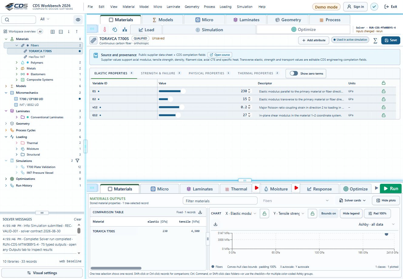
1. Begin with material units, density, elastic constants and strength allowables. Starter values are representative—not certified design allowables. See screenshot
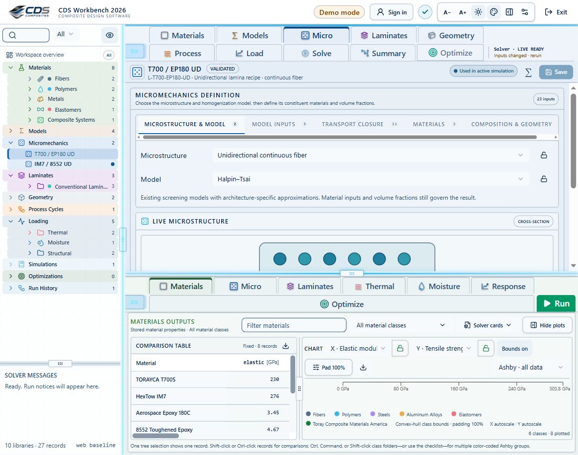
2. Choose the microstructure and compatible model, then constituents, volume fractions and geometric inputs. Check the live cross-section and effective properties. See screenshot
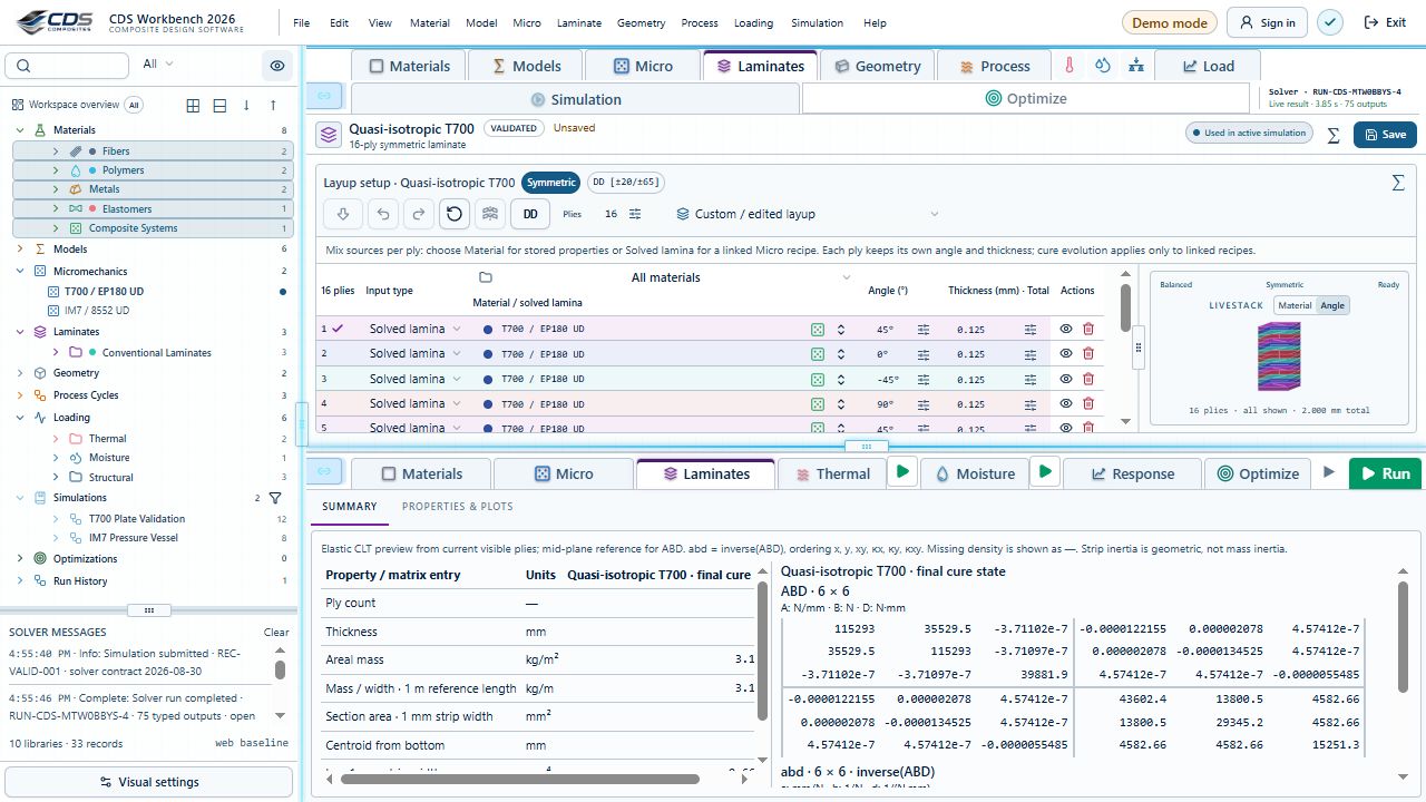
3. Build the laminate: verify source, angle, thickness, ordering, symmetry, balance and visible plies. See screenshot
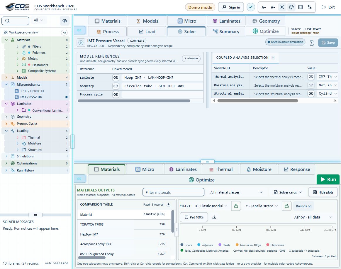
4. Link the applicable geometry and laminate inside each case. Choose the case combination in SIMULATION and review Summary before Run. See screenshot
5. Save a dependency-complete CDS_DB checkpoint so references travel with the study.

Live sync: navigation and calculation are different

Inputs and Outputs have independent menu-response controls. With a control enabled, selecting a tree record updates that pane. Turn one off to keep its current view while navigating the other. An explicit open/double-click can open the chosen record even when ordinary menu response is off.

1. Use the Inputs/Outputs link controls to decide which pane follows tree selection. See screenshot
2. Use Ctrl/Command-click or Shift-click for comparison selections; check the selected record names, not just the active tab.
3. Drag the main and internal dividers to allocate space. Plot resizing changes presentation, not numerical fidelity. See screenshot

Know whether you are viewing live or saved results

Live CLT uses the current visible ply materials, thicknesses, angles and mechanical loads. A material change can therefore update elastic stress/strain previews without a full service run. Thermal, cure and moisture residuals may still come from the last saved solver run.

1. Read the response source and process-time controls in Response. Combined, mechanical and environmental contributions are different views.
2. After changing a material, laminate or process history, rerun the solver before relying on coupled residual results.
3. Treat Inputs changed, rerun, incomplete inputs and unavailable-contribution messages as part of the result—not cosmetic warnings.
4. Use Run History to identify the completed run and its messages. Save input records and export the complete study when it becomes a review baseline.

Material classes, icons and searchable selection

Built-in material classes have stable visual identities: fibers, polymers, hexagonal cores, metal ingots, elastomer dogbones and green composite microstructure icons. User-defined classes can have a selected icon and color. A new material also needs a material type because type determines its input records.

1. Search the laminate material selector by material or class. Use the All materials filter above Material / solved lamina to narrow long lists.
2. Confirm the full material name and source type before selecting a ply source. Color helps recognition; it is not a substitute for identity or units.
3. Use a selected column’s fill-down arrow to copy the selected row’s value. Review the affected plies before saving.
4. Use Duplicate and enter a count for design studies. Copies get separate identities; linked records remain references unless separately duplicated.

Keep sources and completion assumptions visible

Material records can store a source URL, citation, status, basis and notes. Supplier-supported values and CDS engineering completion fields remain distinguishable in the same record.

1. Open Source and provenance above the material property groups and follow any supplier links. Multiple source links are shown separately. See screenshot
2. Use Show zero terms when a stored zero-value property needs to be reviewed or edited. Zero does not mean unavailable; confirm its physical meaning. See screenshot
3. Treat public supplier values, internal qualified records, representative starter values and model fallbacks as different evidence levels.
4. When a material lacks a required transport or strength property, enter qualified data or use an explicitly visible editable model input. Do not assume a successful solve proves the source material record was complete.

Move and duplicate study records in groups

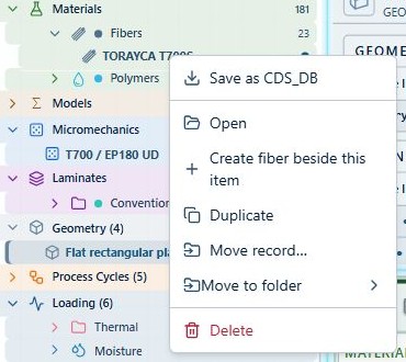
Multi-selection applies to records throughout the master tree. This supports design-study setup without repeating the same move or duplicate command one item at a time.

1. Select records with Ctrl/Command-click or a contiguous range with Shift-click.
2. Choose Move, search for a compatible destination class, review the count and confirm the operation. See screenshot
3. Choose Duplicate and enter the required copy count. Each copy receives its own identity. See screenshot
4. The Optimizations branch remains visible under Simulations even when empty. Saved laminate, lamina/micro and process studies appear there for reopening and comparison.

Laminate construction and LiveStack

The ply table and LiveStack share the same layup. The material and angle color modes answer different questions: which material is used, and how fibers are oriented. Presets, symmetry, balance and Double-Double actions change the layup and must be reviewed as engineering edits.

1. Check the ply count, total thickness and source material after a preset or fill operation. See screenshot
2. Use the geometry-type dropdown to expose the relevant dimensions. Per-type values are retained when changing types.
3. Inspect laminate properties alongside ABD and inverse-ABD matrices. Off-diagonal coupling can be real; it is not automatically an error.
4. A hidden ply is excluded from the current visible-ply preview. Resolve hidden plies before optimization rather than silently optimizing a different stack. See screenshot

Independent boundaries and shared pressure

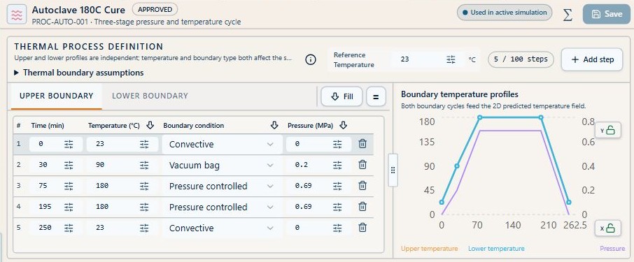
Upper and lower thermal boundary schedules can differ. Their time, temperature and boundary condition records define the applied history. Pressure shown alongside both boundary tables is a shared process load—not two independent pressures to add together.

1. Define ordered cycle steps and check units before using Temperature, boundary-condition or pressure fill-down. See screenshot
2. Set the thermal or moisture analysis resolution and output interval in its input record. See screenshot
3. Use the solver-level 2D grid. The former coarse display grid has been removed; the default 51 × 33 example reflects its time and through-thickness settings, not a universal mesh.
4. Inspect the 2D history with time-history and through-thickness sections alongside it. Move the cursor to examine a matching time/depth state.
5. Check film coefficients, initial conditions and any missing heat-of-reaction or kinetic-model messages before interpreting residual stress.

Compare, preserve and reopen evidence

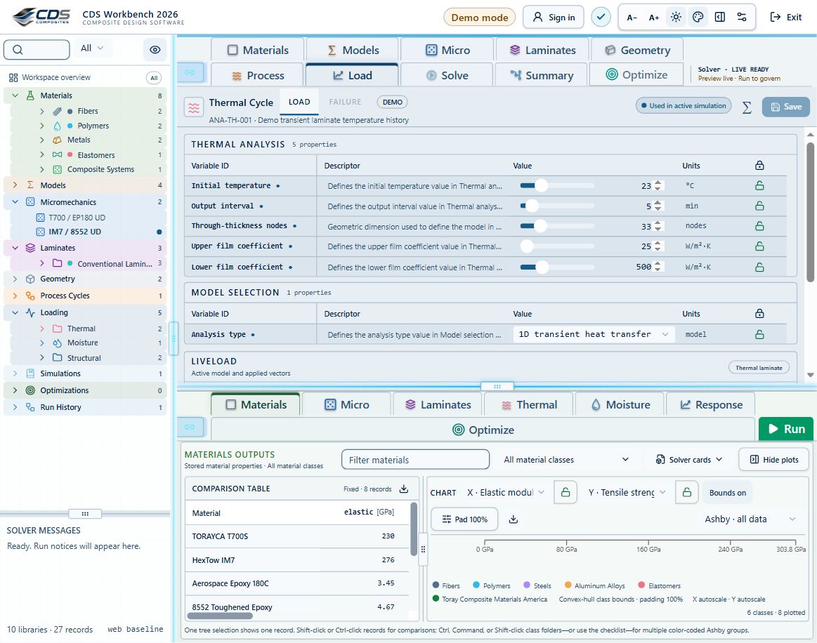
Materials and saved optimization cases offer a comparison table and Ashby, bar and line plots. Axes, units, filtering, markers and bounds control what is shown; they do not change the source calculations.

1. Choose comparable properties and compatible units before comparing records.
2. Use plot bounds and axis locks deliberately; a locked axis can hide an out-of-range point.
3. Save a record, subtree or workspace as CDS_DB for portability. Keep the dependent material, model, laminate, geometry and case records.
4. Save optimization results with Save snapshot beside the structural-case selector. Open saved cases from the permanent Optimizations tree entry below Simulations.
5. Select multiple optimization snapshots to compare them. A saved case is read-only evidence of its saved inputs, not a fresh solve against current materials.