
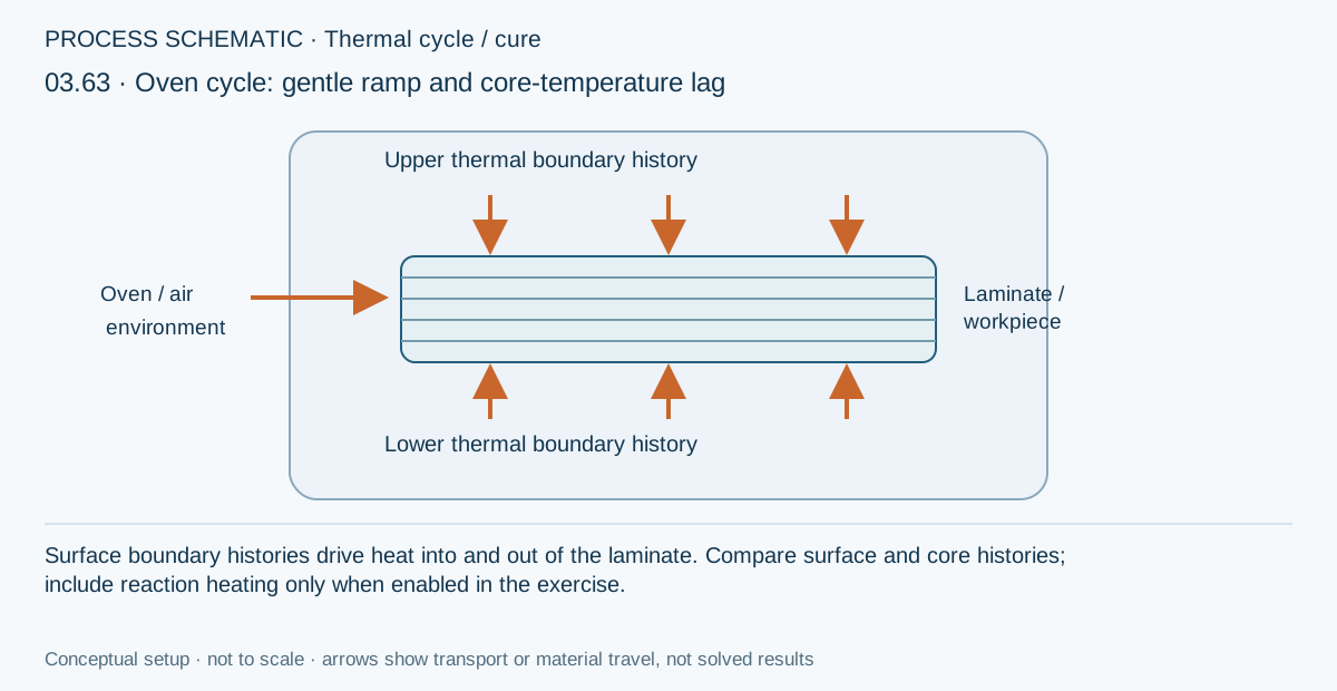
The environment’s temperature schedule and the temperature inside a laminate are not the same history. This exercise follows heat transfer through the thickness and, where enabled, the contribution from resin reaction heat, so that the surface and core can be interpreted as parts of one evolving process.
Open this exercise in Workbench
Prepare the baseline
Inspect the initial temperature, surface conditions, schedule and linked material data before running. Use the baseline to identify ramp, dwell and cooling intervals, then make the prescribed comparison while keeping unrelated parameters fixed. For a reaction-on versus reaction-off comparison, retain the distinction between a diagnostic calculation and a physically calibrated process model.
Worked procedure
1. Open Thermal → Ovens and inspect the air-temperature schedule, convection coefficients and linked laminate. Temperatures are prescribed air boundaries, not the core temperature.
2. Run the active simulation. Compare upper surface, core and lower surface temperature through ramp, dwell and cooling. Inspect the linked cure model and reaction heating.
3. Double the ramp duration in a separate copy, keep dwell temperatures fixed and compare core lag and peak temperature.
4. Repeat with 65 thickness nodes. Record final conversion and core temperature; increase cooling time if the part has not returned to its reference temperature.
Review checkpoints
The schedule uses minutes and zero applied pressure. This is an oven boundary study, not an airflow or equipment model.
Distinguish air setpoint, part temperature and exothermic overshoot.
A completed run is not proof of a qualified cure; compare time and mesh sensitivity.
Model limits
Illustrative oven schedules and convection coefficients using teaching laminate and cure data. One-dimensional thickness transport; no oven airflow, radiation exchange, tooling thermal mass or equipment control model. Calibrate material kinetics and boundary conditions before manufacturing use.
Interpret the comparison
Read the complete history rather than only the final contour. Compare core lag, internal peaks and gradients at stated times, and check the relevant temporal and thickness refinement. If residual stress is discussed, first establish the cooled reference state; a peak stress during processing is not necessarily the stress remaining after cooling.
How information passes between models
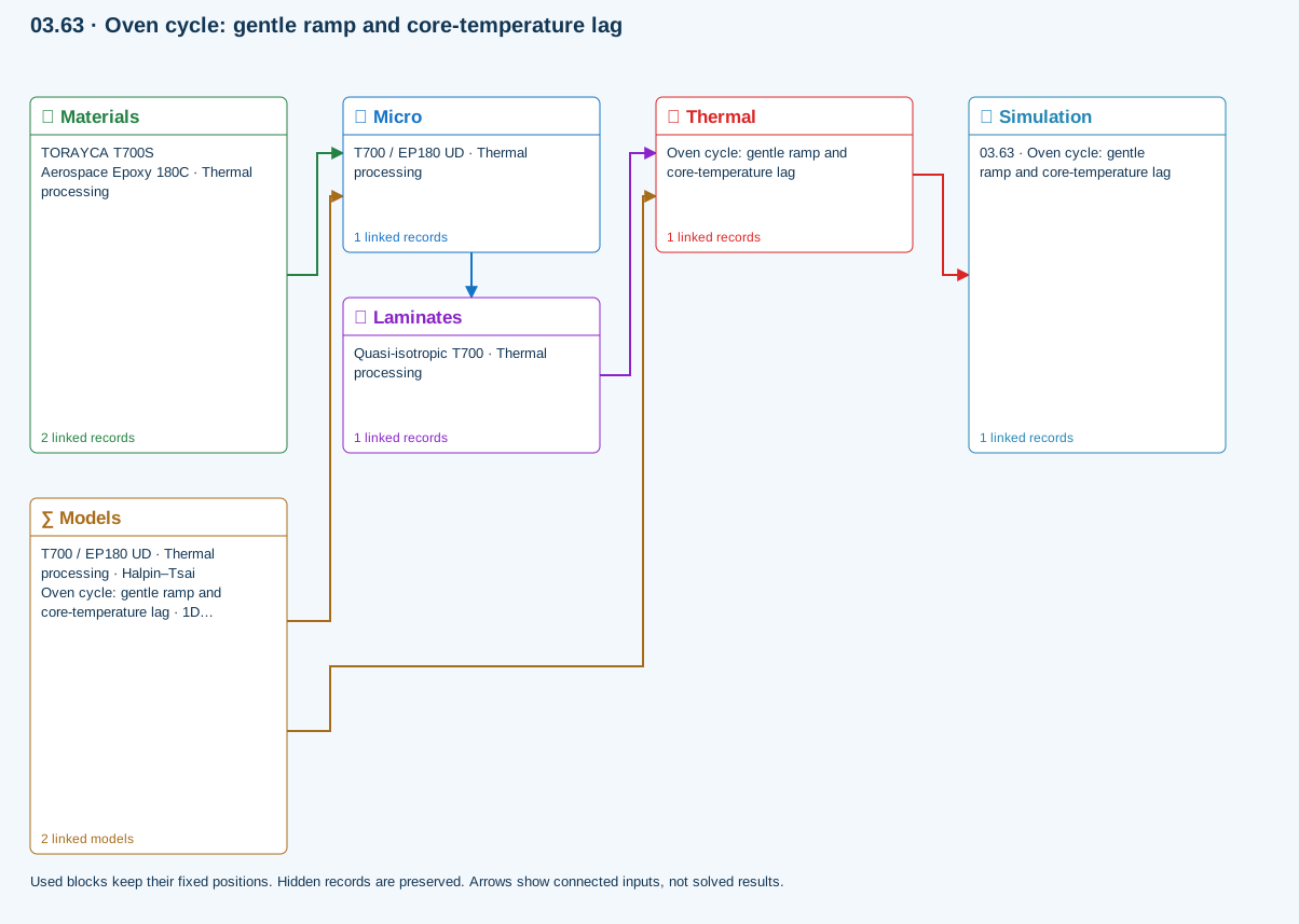
Micro → Laminates: Predicted ply stiffness, strength, density and expansion properties.
Materials → Micro: Constituent stiffness, strength, density and thermal / moisture properties.
Thermal → Simulation: SIMULATION selects this case and its analysis model; the case owns its applicable cycle and input references.
Laminates → Thermal: Ply angles and thicknesses, stiffness, mass and ply properties.
Models → Micro: Applied model assignment: Halpin–Tsai. Model parameters and formulation are used by Micro.
Models → Thermal: Applied model assignment: 1D transient heat transfer. Model parameters and formulation are used by Thermal.
Further reading and evidence
- Enter a process cycle and boundary conditions
- Edit material properties and units
- Run and review a model
- Cure exotherm and evolving modulus
- Connected inputs and result freshness
- Related case study: NASA process cure
Review the recorded validation scope. Retain the original inputs and solver notices with the results. Representative teaching data are not design allowables.
References and source sections
References are retained with the formulations they support. Software instructions describe implementation scope; a cited source does not establish independent validation of a CDS calculation.