
Tool release asks what shape a laminate adopts under the prescribed free-strain assumptions after constraint is removed. This exercise examines that separate analytical question and distinguishes flat-laminate curvature from a corner spring-in estimate.
Illustrative calibration only. Start with a 16-ply cross-ply reference laminate; this is a separate, reference-state study.
Open this exercise in Workbench
Prepare the baseline
Inspect the laminate and the prescribed temperature, expansion and effective shrinkage inputs. Check their reference state and interpretation before running. Vary one supported input in a copy and compare the corresponding shape measure, preserving the rest of the geometry and material assumptions.
Worked procedure
1. Follow the study’s laminate link and inspect the stack and resolved properties that it will use. Then read the model scope and identify the additional specimen, loading or calibration inputs belonging to this separate study. Record which values are supplied independently rather than assuming that every required quantity is inherited from the laminate.
2. Run the supplied study as a baseline and inspect the complete response curves, including their axes, units and parameter settings. Retain the numerical values or a clearly labelled capture before changing an input. Use the interpretation guidance below and the linked formulation to identify what each curve represents and which conclusions remain outside its scope.
3. Choose one editable parameter that belongs to this model and record its original and revised values. Keep the other inputs fixed, rerun the study, and compare the same output quantities over the same range. Explain the observed change using the linked formulation, including a discussion of whether the comparison stays within the model’s calibration and assumptions.
Review checkpoints
Do not interpret example calibration values as material allowables.
Record the assumptions and distinguish analytical verification from experimental validation.
Model limits
Free CLT release from prescribed ply-local shrinkage/thermal eigenstrains. Corner spring-in is a separate uniform-strain estimate. Stress-free temperature and effective post-gel shrinkage need calibration. No tool friction, cure kinetics or viscoelastic restraint history.
Interpret the comparison
Explain the predicted shape using the free strains and laminate coupling in this study. Do not describe it as a resolved tool-contact, friction or viscoelastic cure-history calculation. The model uses prescribed effective strains rather than automatically importing a cure trajectory, and that distinction belongs in the saved conclusion.
How information passes between models
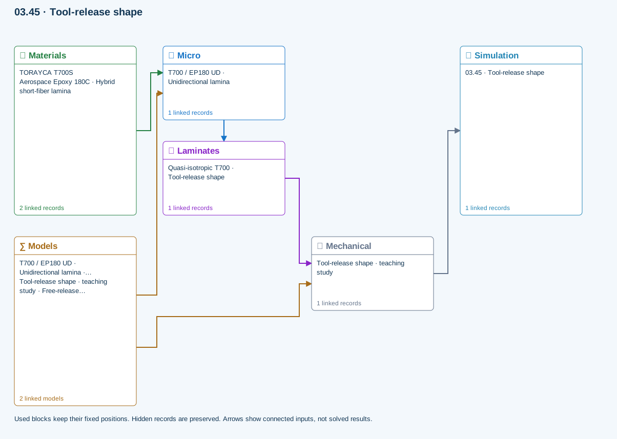
Micro → Laminates: Predicted ply stiffness, strength, density and expansion properties.
Materials → Micro: Constituent stiffness, strength, density and thermal / moisture properties.
Mechanical → Simulation: SIMULATION selects this case and its analysis model; the case owns its applicable cycle and input references.
Laminates → Mechanical: Ply angles and thicknesses, stiffness, mass and ply properties.
Models → Micro: Applied model assignment: Halpin–Tsai. Model parameters and formulation are used by Micro.
Models → Mechanical: Applied model assignment: Free-release eigenstrain & spring-in. Model parameters and formulation are used by Mechanical.
Further reading and evidence
- Advanced analytical models: equations, calibration and limits
- Edit laminate materials, angles and thicknesses
- Run and review a model
- Connected inputs and result freshness
Review the recorded validation scope. Retain the original inputs and solver notices with the results. Representative teaching data are not design allowables.
References and source sections
References are retained with the formulations they support. Software instructions describe implementation scope; a cited source does not establish independent validation of a CDS calculation.